Data Collection

The dataset used is the movie dataset downloaded from Kaggle called the movie database(TMDB). The objective of the analysis was to find out useful insights from the dataset. Python was used for this analysis.

Data Assess

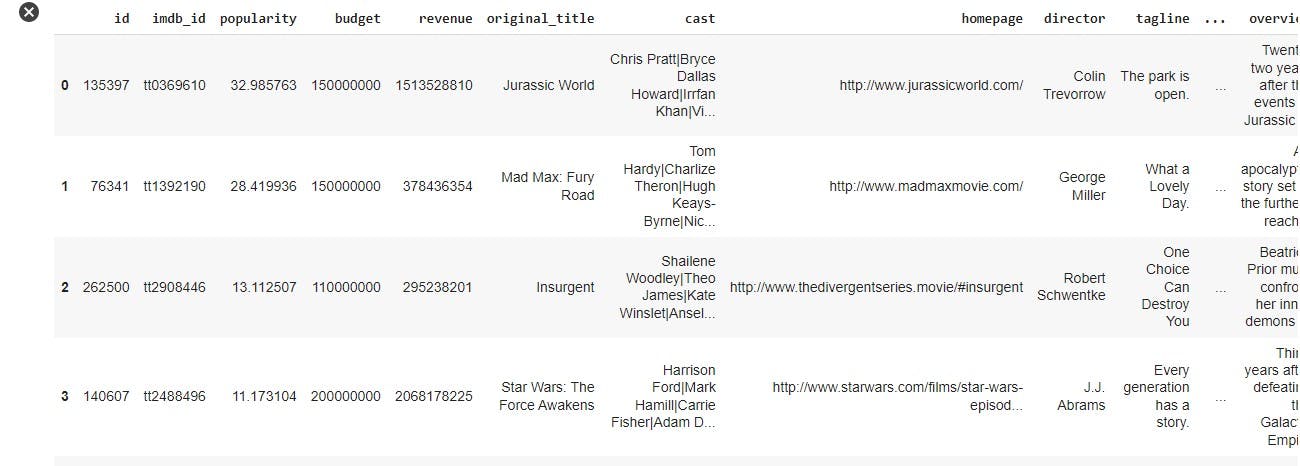
The necessary modules were imported; pandas, numpy, matplotlib, and seaborn. The csv file was then converted to dataframe and then the first five rows and columns were then displayed.

#import the modules
import pandas as pd
import numpy as np
import matplotlib.pyplot as plt
import seaborn as sns
%matplotlib inline

#load the movie dataset
df_movie = pd.read_csv('movies.csv')
df_movie.head()

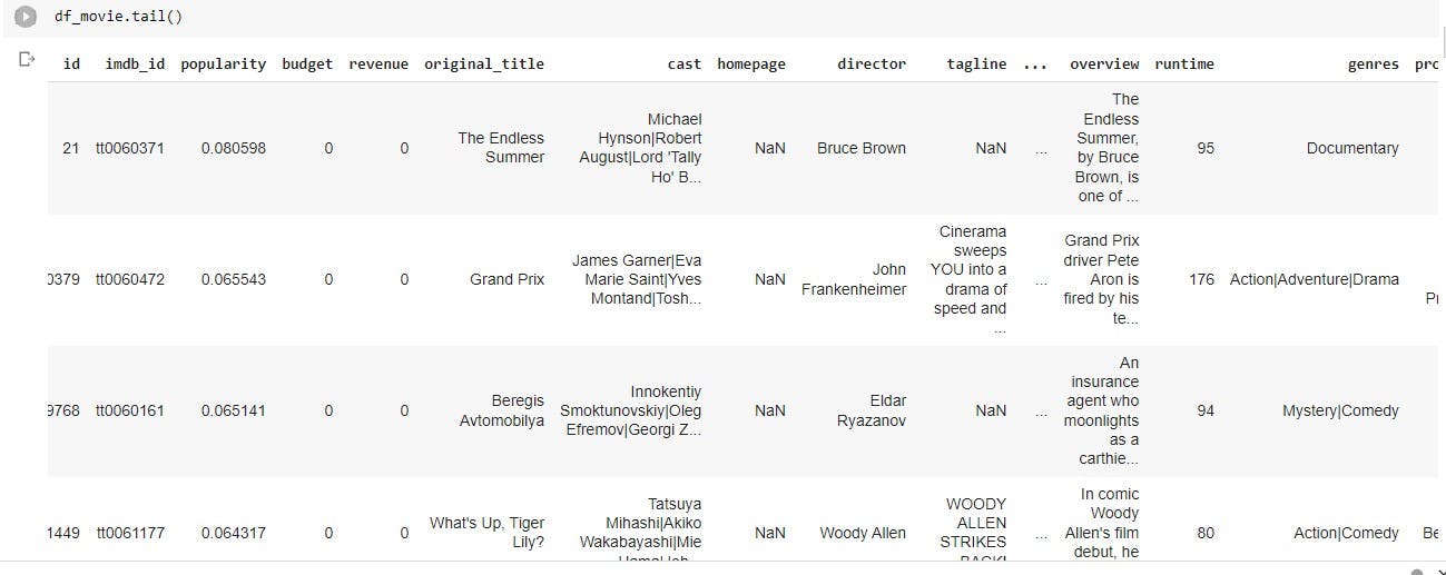
The tail of the dataframe is also viewed

df_movie.tail()

The number of rows and columns were determined. The dataset had 10866 rows and 21 columns.

df_movie.shape

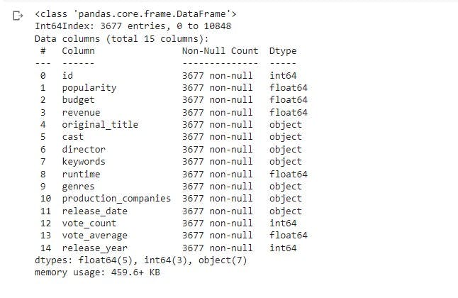
To know the broad information of the dataset such as the number of not null values for each column, and the data type of each column. I used the info() method.

df_movie.info()

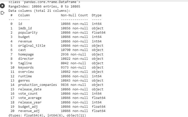
From the overview, observations were made:

• In the genre column, there was more than one genre for each movie.
• The dataset had a lot of null values that had to be investigated and acted upon.
• Some columns will have to dropped as they were not necessary for this analysis.

Data Cleaning

Duplicates were checked and removed from the dataframe and the columns which were not necessary for the analysis were dropped. Null values were also checked and replaced with zero values and then dropped.

df_movie.duplicated().sum()

df_movie.drop_duplicates(inplace=True)
df_movie.drop(['budget_adj','revenue_adj','overview','imdb_id','homepage','tagline'],axis =1,inplace = True)

df_movie.isna().sum()

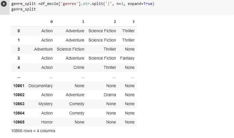
The genre column had one or more genre for a movie so it was then split so that it would be analyzed easier.

Checking the dataframe information again one would see the effect of the cleaning.

df_movie.info()

Exploratory Data Analysis: Insights from the data

This is the part to get insights from the data such as;

1. Which is the most popular genre annually?
2. What kind of properties are associated with movies that high revenues?
3. How many movies are produced annually?
4. Movies with the highest budget
5. Top 10 movies with the highest revenue.
6. 10 most popular movies
7. 10 most profitable movies
8. 10 Least profitable movies.
9. Genres with the highest release.

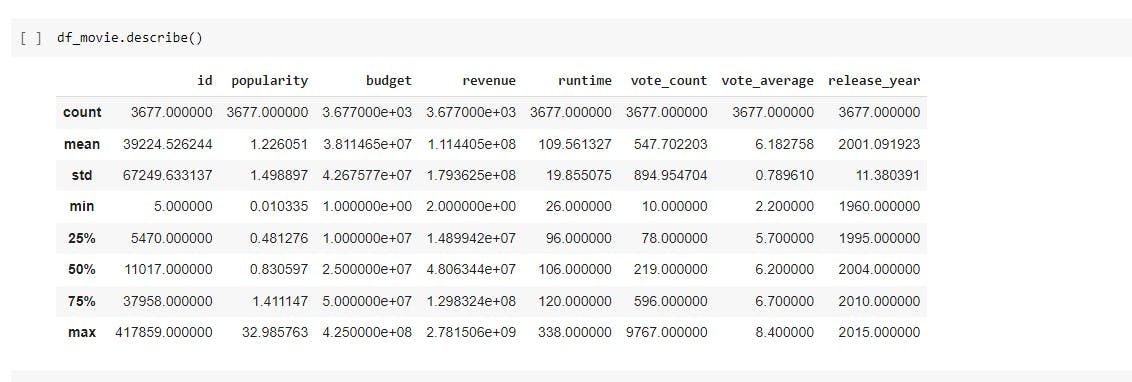
The first thing I like to do after cleaning is to summarize the characteristics of the numeric part of the dataset. This shows the minimum, maximum, mean, standard deviation, median, 25% and 75th percentile.

df_movie.describe()

Which of the genre that was released was most popular yearly? First thing is to know how many genres that are in the dataset.

def separate_count(column):
    genre_split = pd.Series(df_movie[column].str.cat(sep = '|').split('|'))

    genre = list(genre_split.unique())
    #genre2 = genre.replace(' ',',')
    return  genre

genre = separate_count('genres')

print(genre)

There were twenty genres in the dataset.

'Action', 'Adventure', 'Science Fiction', 'Thriller', 'Fantasy', 'Crime', 'Western', 'Drama', 'Family', 'Animation', 'Comedy', 'Mystery', 'Romance', 'War', 'History', 'Music', 'Horror', 'Documentary', 'Foreign', 'TV Movie'

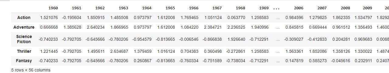
Create a list from the genre column and put into a variable. Create numpy array of year and popularity and create variables them. Then create a dataframe where the index is the genres and the columns are years. The range year is between the minimum year and the maximum year according to the descriptive statistics for the release year. Search through the split genre and determine the popularity of a genre by the release year using a for loop.

genre_list = list(map(str,(df_movie['genres'])))


#make the numpy array of year and popularity which contain all the rows of release_year and popularity column. 
year = np.array(df_movie['release_year'])
film_popularity = np.array(df_movie['popularity'])

#make a null dataframe which indexs are genres and columns are years.
df_popular = pd.DataFrame(index = genre, columns = range(1960, 2016))
#The range year is between the min year and the max year according to the descriptive statistics for release year.
#change all the values of the dataframe from NAN to zero.
df_popular = df_popular.fillna(value = 0.0)

x = 0
for y in genre_list:
    split_genre = list(map(str,y.split('|')))
    df_popular.loc[split_genre, year[x]] = df_popular.loc[split_genre, year[x]] + film_popularity[x]
    x+=1

Create a function to calculate the standard deviation of the popular genre.

def calculate(x):
    return (x-x.mean())/x.std(ddof=0)

popular_gen = calculate(df_popular)

Create a bar plot of the standardized data.

#plot the bar plot of the standardised data.
popular_gen.iloc[0:,53:].plot(kind='bar',figsize = (15,6),fontsize=13)


#setup the title and labels of the plot. 
plt.title("Most Popular Genre Over Year To Year",fontsize=15)
plt.xlabel("Popularity",fontsize=15)
plt.ylabel("Genres",fontsize = 15)

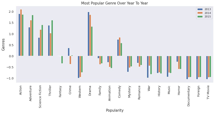From the image above, the most popular genres are action, Thriller and adventure respectively.

For a more clear view of the twenty genre and how they trended each year,

#plot the barh plot of the standardised data.
popular_gen.iloc[0:,53:].plot(kind='bar',figsize = (15,6),fontsize=13)


#setup the title and labels of the plot. 
plt.title("Most Popular Genre Over Year To Year",fontsize=15)
plt.xlabel("Popularity",fontsize=15)
plt.ylabel("Genres",fontsize = 15)

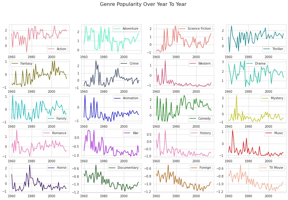
The line plots is a more comprehensive data showing the popularity of a genre from year to year. There are twenty genres in this data set. The year range is from 1960-2015. It shows the popularity from Action genre to TV Movie genre.

One would notice that there is a spike in the 60s for almost all the genres. One would also notice that the top three popular genres here are Action, Adventure and thriller. Science Fiction follows closely behind in the fourth position.

2. Properties associated with movies that have high revenues What made the movies to have higher profits. According to the datasets the columns involved are budget, popularity, vote_average and the runtime. The budget is the financial cost of making a movie. The popularity is the degree of likes and high rating the movie makes after it has been released. The vote_average is the rating of the movie by viewers and the run_time is how long the movie runs from start to finish.

revenue = pd.DataFrame(df_movie['revenue'].sort_values(ascending=False))
movie_properties =
 ['id','popularity','budget','original_title','cast','director','runtime','genres','vote_average','release_year']
for i in movie_properties:
    revenue[i] = df_movie[i]

Creating a regression plot to determine the linear relationship between the revenue and the other columns. one would observe that the budget and popularity has a stronger linear relationship than the other two with the revenue.

fig, axes = plt.subplots(2,2,figsize = (16,6))
fig.suptitle("Revenue Vs (Budget,Popularity,Vote Average,Runtime)",fontsize=14)

sns.regplot(x=df_movie['revenue'], y=df_movie['budget'],color='b',ax=axes[0][0])
sns.regplot(x=df_movie['revenue'], y=df_movie['popularity'],color='b',ax=axes[0][1])
sns.regplot(x=df_movie['revenue'], y=df_movie['vote_average'],color='b',ax=axes[1][0])
sns.regplot(x=df_movie['revenue'], y=df_movie['runtime'],color='b',ax=axes[1][1])

sns.set_style("dark")

To further buttress this, I used a heatmap to find the correlation score.

df = pd.DataFrame(df_movie,columns=['popularity','budget','revenue','runtime','vote_count','vote_average'])
corrMatrix = df.corr()
sns.heatmap(corrMatrix, annot=True)
plt.show()

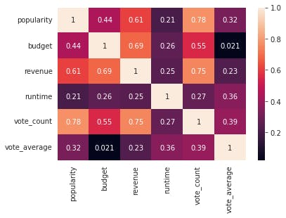In the image above, the highest correlation score is 0.75 which is the Vote_count versus the revenue. This is followed by the budget with a score of 0.69, popularity is the third with a score 0.61.

3. Number of movies released annually

# make group for each year and count the number of movies in each year 
movie_number=df_movie.groupby('release_year').count()['id']
print(movie_number.tail(10))

#make group of the data according to their release year and count the total number of movies in each year and pot.
df_movie.groupby('release_year').count()['id'].plot(xticks = np.arange(1960,2016,5))

#set the figure size and labels
sns.set(rc={'figure.figsize':(10,5)})
plt.title("Year Vs Number Of Movies",fontsize = 14)
plt.xlabel('Release year',fontsize = 13)
plt.ylabel('Number Of Movies',fontsize = 13)
#set the style sheet
sns.set_style("dark")

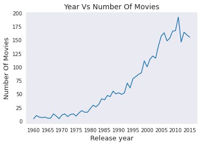The highest number of movies was released in 2011 with 192 movies in total. The second highest was in 2009 with 166 movies.

4. Movies with the highest budget

budget=  pd.DataFrame(df_movie['budget'].sort_values(ascending = False))
budget['original_title'] =df_movie['original_title']
data = list(map(str,(budget['original_title'])))
x = list(budget['budget'][:10])
y =list(data[:10])
sns.lineplot( x=x, y=y)
plt.title("Movies with the highest Bugdet")
plt.xlabel("Budget")
plt.ylabel("Movie Title")

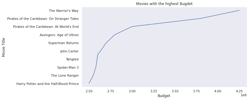The the top three movies with the highest budget, the warrior way, pirate of the carribean: Stranger tides and The world's end.

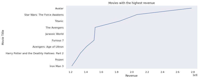
5. Movies with the highest revenue

revenue =  pd.DataFrame(df_movie['revenue'].sort_values(ascending = False))
revenue['original_title'] =df_movie['original_title']
data = list(map(str,(revenue['original_title'])))
x = list(revenue['revenue'][:10])
y =list(data[:10])
sns.lineplot( x=x, y=y)
plt.title("Movies with the highest revenue")
plt.xlabel("Revenue")
plt.ylabel("Movie Title")

6. Top 10 most popular movies

popular =  pd.DataFrame(df_movie['popularity'].sort_values(ascending = False))
popular['original_title'] =df_movie['original_title']
data = list(map(str,(popular['original_title'])))
x = list(popular['popularity'][:10])

y =list(data[:10])
sns.lineplot( x=x, y=y)
plt.title("Top 10 Most Popular Movies")
plt.xlabel("Popularity")
plt.ylabel("Movie Title")

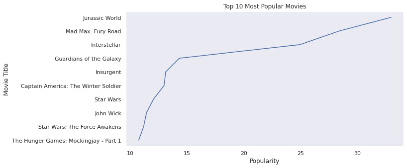The most popular films are Jurassic world, Mad Max fury and Interstellar.

1. Top 10 profitable movies

df_movie['Profit'] = df_movie['revenue'] - df_movie['budget']
profit = pd.DataFrame(df_movie['Profit'].sort_values(ascending = False))
profit['original_title'] = df_movie['original_title']
data = list(map(str,(profit['original_title'])))
title= list(data[:10])
highgross = list(profit['Profit'][:10])
sns.lineplot( x=highgross, y=title)
plt.title("Top 10 Profitable movies")
plt.xlabel("Profit")
plt.ylabel("Movie Title")

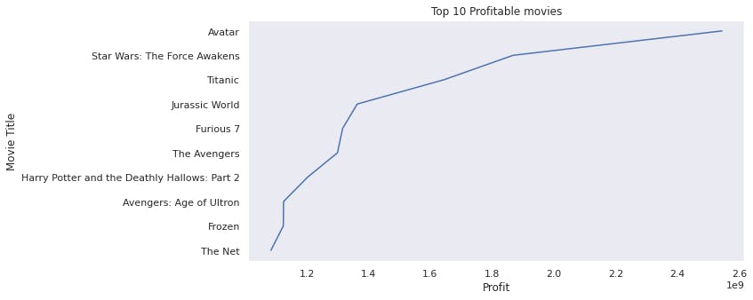Avatar is the highest profitable movie followed by Starwars, Titanic and Jurassic world.

8. Top 10 least profitable movies

least_profit = pd.DataFrame(df_movie['Profit'].sort_values(ascending = True))
least_profit['original_title'] = df_movie['original_title']
data = list(map(str,(least_profit['original_title'])))
high_Gross = list(data[:10])
title = list(least_profit['Profit'][:10])
ax = sns.lineplot( x=title, y=high_Gross)
plt.title("Movies with the least profit")
plt.xlabel("Least Profit")
plt.ylabel("Movie Title")

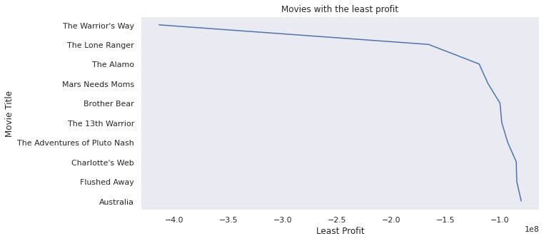The lowest grossing movie is Warrior way followed by Lone Ranger, Alamo and Mars need Moms.

9. Genre with the highest release

def calculate(x):
    #concatenate all the rows of the genrs.
    genre_plot = df_movie[x].str.cat(sep = '|')
    data = pd.Series(genre_plot.split('|'))

    info = data.value_counts(ascending=False)
    return info

#call the function for counting the movies of each genre.
total_genre_movies = calculate('genres')

total_genre_movies.plot(kind= 'bar',figsize = (13,6))

#setup the title and the labels of the plot.
plt.title("Genre With Highest Release",fontsize=15)
plt.xlabel('Number Of Movies',fontsize=13)
plt.ylabel("Genres",fontsize= 13)
sns.set_style("dark")

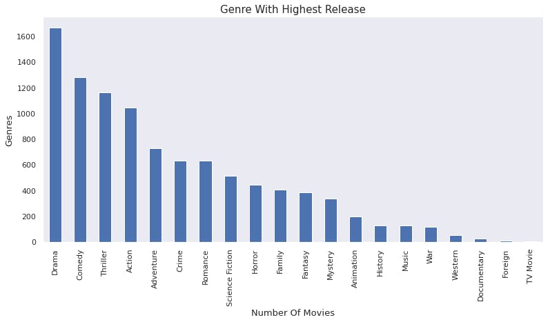Drama has the highest release of genre followed by comedy

Conclusions

1. Action is the most popular movie produced annually.
2. vote_count was hightly correlated to the revenue with a correlation score of 0.71 followed by budget with a correlation score of 0.69
3. Year 2011 had the highest amount of movies produced with 192 movies released.
4. The movie with the highest budget is The Warrior's way followed by Pirates of the Carribean: On Stranger Tides.
5. The movie that has the highest revenue is Avatar followed by Star Wars and Titanic.
6. The most popular movie is Jurassic World followed by Mad Max
7. The most profitable movie is Avatar.
8. The least profitable movie is The Warrior Way. Even though it had the highest budget, it still did not make it profitable.
9. Genre with the highest release is Drama followed by the Comedy genre.

Limitations

• One would see from the datasets. In the beginning of the investigation, there were about 10,000 datasets, but to get insights from the data. we had to delete the null data which would have affected the results leaving a little less than 4000 movie datasets.
• The genre had a seperator character("|") which had to be split during the data cleaning process. To investigate the data in this category took longer time than if it did not have this character.