INTRODUCTION

In data science, statistics is at the core of sophisticated machine learning algorithms, capturing and translating data patterns into actionable evidence. Data scientists use statistics to gather, review, analyze, and draw conclusions from data, as well as apply quantified mathematical models to appropriate variables. There are two types of data; the quantitative and the qualitative data. Quantitative is also known as numeric data while qualitative is also known as categorical data.

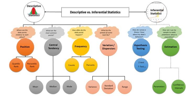
Statistics can be grouped into two main types; Descriptive and Inferential statistics.

Descriptive Statistics

This describes and summarizes the data at hand. It does that in three forms; central tendency, spread and distribution. I will go to these characteristics later.

Inferential Statistics

This uses a sample of data to make inferences about a larger population. For example what percentage of people drive to work in your area. Inferential statistics come from a general family of statistical model know as the General Linear model. This includes the t-test, Analysis of Variance (ANOVA), Analysis of Covariance (ANCOVA), Chi-squared, Regression Analysis, Cluster Analysis e.t.c.

Image by Datacentral

Types of Descriptive Statistics

Measures of central tendency

This attempts the describe the set of data by identifying the central position within that data. There are three measures of central tendency; mean, median and the mode.

Mean: This is the sum of the values /total number of values.

Median: This is the middle number in an ordered data set.

Mode: This is the most frequent value in the dataset.

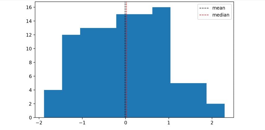
In a symmetrical data, the mean, median are about the same thing.

Image by Datacamp

For a skewed data, the median is not equal to the mean and the data is asymmetrical

Image by Datacamp

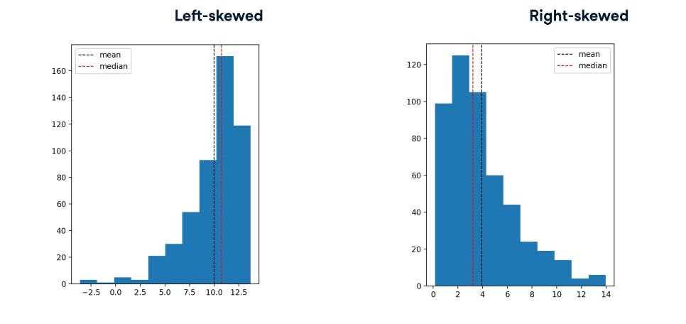
When to use which measure: When the data is symmetrical, the mean can be used. Median is used as a measure when the data is skewed.

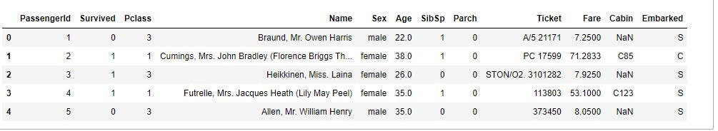
Using an example; the legendary Titanic dataset from kaggle. The data is about information of passengers that boarded the fated ship in April, 1912.

import pandas as pd
import numpy as np
import matplotlib.pyplot as plt
import seaborn as sns
% matplotlib inline

df_titanic =pd.read_csv("datasets/titanic_train.csv")
df_titanic.head()

To check the number of rows and columns, datatype of each of the columns and number of non-null values of the same

df_titanic.info()

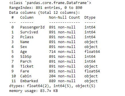
In the above image, you would see that the columns Age, Embarked and Cabin had null values. The last two columns mentioned are string values hence we cannot used it to find the mean or median. The column "Age" is numeric, hence one can the the type of distribution using a histogram plot

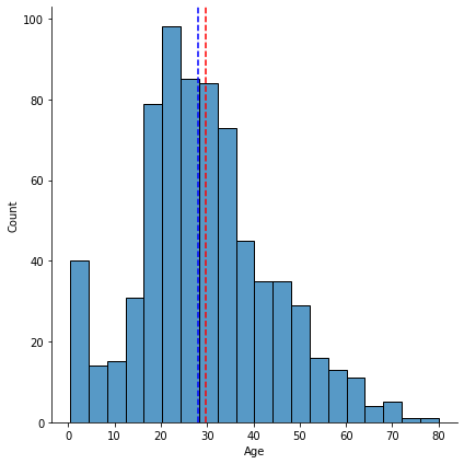
sns.displot(x='Age',data=df_titanic,height=6, bins=20)
plt.axvline(x=df_titanic.Age.mean(),color='red',linestyle='dashed')
plt.axvline(x=df_titanic.Age.median(),color='blue',linestyle='dashed')

plt.show()

Image by Author In the above image, the mean and the median is not near each other. Hence one could use the mean or median to replace the null values.

#fill the null values of the age column by the mean
df_titanic['Age']=df_titanic['Age'].fillna(df_titanic['Age'].mean())

Now to check if there is any null value in the Age column

df_titanic.Age.isnull().sum()

There is none since we have filled the null values with the mean.

Mode is the value with the highest frequency. In this age category, to know the mode of Age, use the value_counts() method.

df_titanic.Age.value_counts()

The age with the highest number of frequency is 24 years. This means more people of 24 years boarded the ill fated ship. Also in the histogram above, one would notice that the peak age is at that value.

Measures of Spread

This describes how spread apart of close the data points are. The measures of spread used are:

• Variance
• Standard Deviation
• Quartiles -Outliers

Variance: This is the average distance between each data point to the mean. For example the variance of the ticket fare of the passengers of the ship np.var(df_titanic['Fare']

Standard deviation: This is the square root of the variance. np.std(df_titanic['Fare']

Quartiles: Quartiles are three values that split sorted data into equal parts, each with an equal number of observations.

np.quartiles(df_titanic['Fare'] [0, 0.25, 0.5, 0.75, 1]))

Inter Quartile Range(IQR): This is the distance between the 25th and 75th percentile. The 50th percentile is also the median.

Outlier: This is when data points are substantially different from each other. A data point is said to be an outlier if data < Q1 - 1.5 IQR or data > Q3 + 1.5 IQR